
Case Study of MixMC sPLS-DA with Koren Bodysite data
The mixMC framework is one that is specifically built for microbial datasets and will be used here on the Koren Bodysite dataset yielded by Koren et al, 2011 [1]. A sPLS-DA methodology will be employed in order to predict the bodysite a given sample was drawn from based on the OTU data (Operational Taxonomic Unit). The model will select the optimal set of OTUs to perform this prediction.
For background information on the mixMC or sPLS-DA methods, refer to the MixMC Method Page and sPLS-DA Method Page.
R script
The R script used for all the analysis in this case study is available here.
To begin
Load the latest version of mixOmics. Note that the seed is set such that all plots can be reproduced. This should not be included in proper use of these functions.
library(mixOmics) # import the mixOmics library

set.seed(5249) # for reproducibility, remove for normal use
The data
The Koren bodysite dataset derives from an examination of the link between oral, gut and plaque microbial communities in patients with atherosclerosis (vs. controls). While the original methodology of this study involved repeated measures, for the sake of simplicity it will be considered as non-repeated for this case study. It is assumed that the data are offset and pre-filtered, as described in mixMC pre-processing steps.
The mixOmics Koren dataset is accessed via Koren.16S and contains the following:
Koren.16S$data.TSS(continuous matrix): 43 rows and 980 columns. The prefiltered
normalised data using Total Sum Scaling normalisation.Koren.16S$data.raw(continuous matrix): 43 rows and 980 columns. The prefiltered raw
count OTU data which include a 1 offset (i.e. no 0 values).Koren.16S$taxonomy(categorical matrix): 980 rows and 7 columns. Contains the taxonomy (ie. Phylum, … Genus, Species) of each OTU.Koren.16S$indiv(categorical matrix): 43 rows and 22 columns. Contains all the sample meta data recorded.Koren.16S$bodysite(categorical vector): factor of length 43 indicating the bodysite with levelsarterial plaque,salivaandstool.
The raw OTU data will be used as predictors (X dataframe) for the bodysite (Y vector). The dimensions of the predictors is confirmed and the distribution of the response vector is observed.
data("Koren.16S") # extract the microbial data
X <- Koren.16S$data.raw # set the raw OTU data as the predictor dataframe
Y <- Koren.16S$bodysite # set the bodysite class as the response vector

dim(X) # check dimensions of predictors
## [1] 43 980
summary(Y) # check distribution of response
## arterial plaque          saliva           stool
##              13              15              15
Initial Analysis
Preliminary Analysis with PCA
The first exploratory step involves using PCA (unsupervised analysis) to observe the general structure and clustering of the data to aid in later analysis. As this data are compositional by nature, a centered log ratio (CLR) transformation needs to be undergone in order to reduce the likelihood of spurious results. This can be done by using the logratio parameter in the PCA function.
Here, a PCA with a sufficiently large number of components (ncomp = 10) is generated to choose the final reduced dimension of the model. Using the 'elbow method' in Figure 1, it seems that two components will be more than sufficient for a PCA model.
koren.pca = pca(X, ncomp = 10, logratio = 'CLR') # undergo PCA with 10 comps

plot(koren.pca) # plot explained variance

FIGURE 1: Bar plot of the proportion of explained variance by each principal component yielded from a PCA.
Below, the samples can be seen projected onto the first two Principal Components (Figure 2). The separation of each bodysite can be clearly seen, even just across these two components (account for a total of 37% of the OTU variation). It seems that the first component is very good at defining the arterial plaque bodysite against the other two bodysites while the second discriminates between the saliva and stool bodysites very well.
koren.pca = pca(X, ncomp = 2, logratio = 'CLR') # undergo PCA with 2 components

plotIndiv(koren.pca, # plot samples projected onto PCs
          ind.names = FALSE, # not showing sample names
          group = Y, # color according to Y
          legend = TRUE,
          title = 'Koren OTUs, PCA Comps 1&2')

FIGURE 2: Sample plots from PCA performed on the Koren OTU data. Samples are projected into the space spanned by the first two components.
Initial sPLS-DA model
The mixMC framework uses the sPLS-DA multivariate analysis from mixOmics [3]. Hence, the next step involves generating a basic PLS-DA model such that it can be tuned and then evaluated. In many cases, the maximum number of components needed is k-1 where k is the number of categories within the outcome vector (y) – which in this case is 3. Once again, the logratio parameter is used here to ensure that the OTU data are transformed into an Euclidean space.
basic.koren.plsda = plsda(X, Y, logratio = 'CLR',
                          ncomp = nlevels(Y))
Tuning sPLS-DA
Selecting the number of components
The ncomp Parameter
To set a baseline from which to compare a tuned model, the performance of the basic model is assessed via the perf() function. Here, a 5-fold, 10-repeat design is utilised. To obtain a more reliable estimation of the error rate, the number of repeats should be increased (between 50 to 100). Figure 3 shows the error rate as more components are added to the model (for all three distance metrics). The Balanced Error Rate (BER) is more appropriate to use here due to the unbalanced response vector (arterial plaque has less samples than the other two bodysites). Across all three distance metrics, a model using three components had the lowest error rate. Hence, it seems that three components is appropriate.
# assess the performance of the sPLS-DA model using repeated CV
basic.koren.perf.plsda = perf(basic.koren.plsda,
                              validation = 'Mfold',
                              folds = 5, nrepeat = 10,
                              progressBar = FALSE)

# extract the optimal component number
optimal.ncomp <- basic.koren.perf.plsda$choice.ncomp["BER", "max.dist"]

plot(basic.koren.perf.plsda, overlay = 'measure', sd=TRUE) # plot this tuning

FIGURE 3: Classification error rates for the basic sPLS-DA model on the Koren OTU data. Includes the standard and balanced error rates across all three distance metrics.
Selecting the number of variables
The keepX Parameter
With the suggestion that ncomp = 3 is the optimal choice, the number of features to use for each of these components needs to be determined (keepX). This will be done via the tune.splsda() function. Again, a 5-fold, 10-repeat cross validation process is used but in reality these values should be higher. Figure 4 below shows that the error rate is minimised when 2 components are included in the sPLS-DA, whereas the third component seems to add noise. The diamonds indicate the optimal keepX variables to select on each component based on the balanced error rate.
Note that the selected ncomp from the tune.splsda() and perf() functions are different. As the sparse model (sPLS-DA) will be used, ncomp = 2 is the more appropriate choice.
grid.keepX = c(seq(5,150, 5))

koren.tune.splsda = tune.splsda(X, Y,
                          ncomp = optimal.ncomp, # use optimal component number
                          logratio = 'CLR', # transform data to euclidean space
                          test.keepX = grid.keepX,
                          validation = c('Mfold'),
                          folds = 5, nrepeat = 10, # use repeated CV
                          dist = 'max.dist', # maximum distance as metric
                          progressBar = FALSE)

# extract the optimal component number and optimal feature count per component
optimal.keepX = koren.tune.splsda$choice.keepX[1:2]
optimal.ncomp = koren.tune.splsda$choice.ncomp$ncomp

plot(koren.tune.splsda) # plot this tuning

FIGURE 4: Tuning keepX for the sPLS-DA performed on the Koren OTU data. Each coloured line represents the balanced error rate (y-axis) per component across all tested keepX values (x-axis) with the standard deviation based on the repeated cross-validation folds.
Final Model
Following this tuning, the final sPLS-DA model can be constructed using these optimised values.
koren.splsda = splsda(X,  Y, logratio= "CLR", # form final sPLS-DA model
                      ncomp = optimal.ncomp,
                      keepX = optimal.keepX)
Plots
Sample Plots
The sample plot found in Figure 5 depicts the projection of the samples onto the first two components of the sPLS-DA model. There is distinct separation of each bodysite as shown by the lack of any overlap of the 95% confidence ellipses.
plotIndiv(koren.splsda,
          comp = c(1,2),
          ind.names = FALSE,
          ellipse = TRUE, # include confidence ellipses
          legend = TRUE,
          legend.title = "Bodysite",
          title = 'Koren OTUs, sPLS-DA Comps 1&2')

FIGURE 5: Sample plots from sPLS-DA performed on the Koren OTU data. Samples are projected into the space spanned by the first two components.
Another way to visualise the similarity of samples is through the use of a clustered image map (CIM). Figure 6 clearly shows which OTUs are associated with a given bodysite. This plot also depicts the sparsity commonly seen in microbial datasets.
cim(koren.splsda,
    comp = c(1,2),
    row.sideColors = color.mixo(Y), # colour rows based on bodysite
    legend = list(legend = c(levels(Y))),
    title = 'Clustered Image Map of Koren Bodysite data')
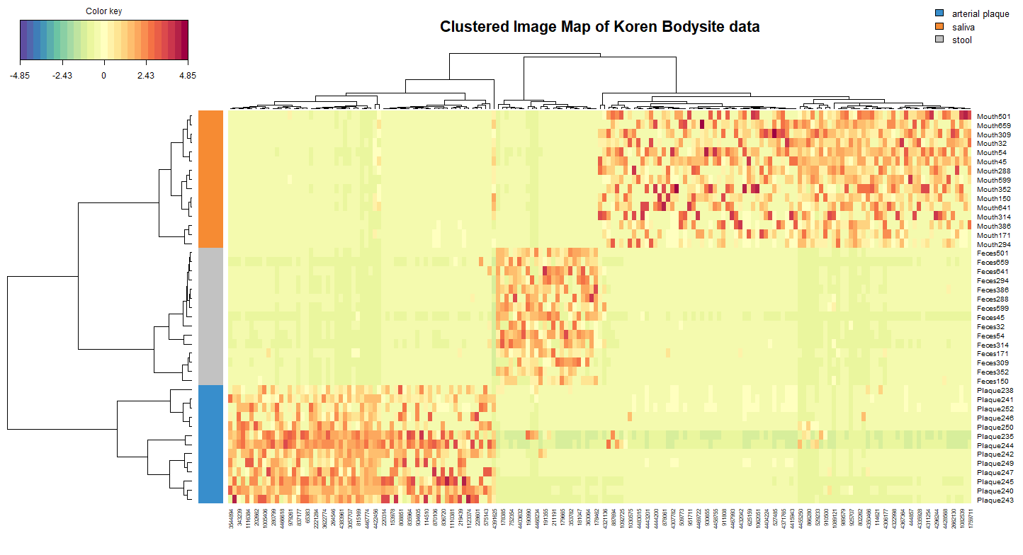
FIGURE 6: Clsutered Image Map of the Koren OTU data after sPLS-DA modelling. Only the keepX selected feature for components 1 and 2 are shown, with the colour of each cell depicting the raw OTU value after a CLR transformation.
Variable Plots
Interpretting Figure 7 below in conjunction with Figure 5 provides key insights into what OTUs are responsible for identifying each bodysite. Note that cutoff = 0.7 such that any feature with a vector length less than 0.7 is not shown. Three distinct clusters of OTUs can be seen – one of each seemingly corresponding to one of the three bodysites. The feature found by itself (4391625) could be interpretted as either:
- being important in the identification of both the
arterial plaqueandsalivabodysites, or - being important in the identification that a sample does not belong to the
stoolbodysite.
plotVar(koren.splsda,
        comp = c(1,2),
        cutoff = 0.7, rad.in = 0.7,
        title = 'Koren OTUs, Correlation Circle Plot Comps 1&2')

FIGURE 7: Correlation circle plot representing the OTUs selected by sPLS-DA performed on the Koren OTU data. Only the OTUs selected by sPLS-DA are shown in components 1 and 2. Cutoff of 0.7 used
The network plot seen in Figure 8 shows furthers the understanding of which OTUs are contributing to each bodysite. For each bodysite, there is a grouping of OTUs which identify that bodysite and none other. There are also two small clusters which contain OTUs which are found at two of the three bodysites, showing a similarity in the microbial communities of these areas. Interestingly, the saliva and arterial plaque bodysites share no common OTUs (at cutoff = 0.5).
network(koren.splsda,
        cutoff = 0.5,
        color.node = c("orange","lightblue"))
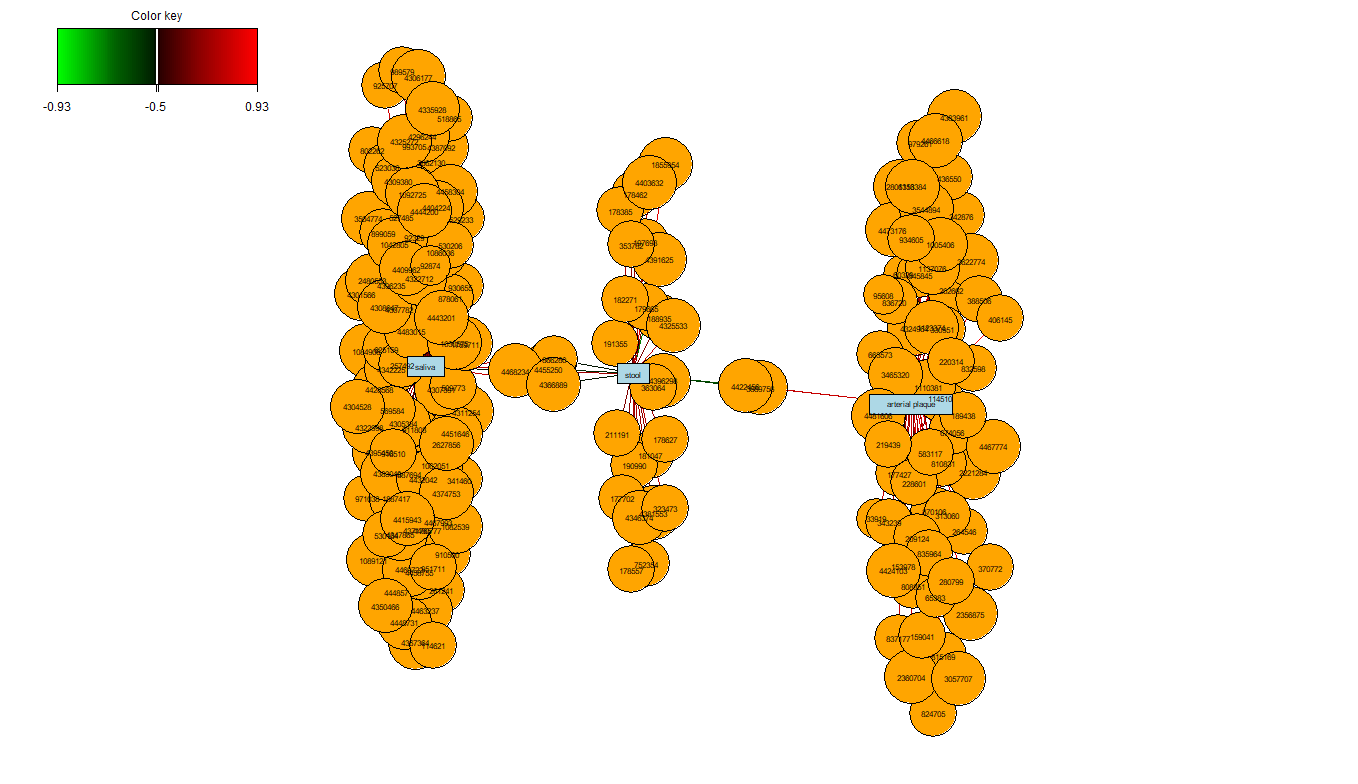
FIGURE 8: Relevance Network graph of the Koren OTUs selected by sPLS-DA on this dataset.
Evaluation of sPLS-DA
The mixOmics package also contains the ability to assess the classification performance of the sPLS-DA model that was constructed via the perf() function once again. The mean error rates per component and the type of distance are output. It can be beneficial to increase the number of repeats for more accurate estimations. It is clear from the below output that adding the second component drastically decreases the error rate.
# for reproducible results for this code, remove for your own code
set.seed(5249)

# evaluate classification, using repeated CV and maximum distance as metric
koren.perf.splsda = perf(koren.splsda, validation = 'Mfold',
                         folds = 5, nrepeat = 10,
                         progressBar = FALSE, dist = 'max.dist')

koren.perf.splsda$error.rate
## $overall
##        max.dist
## comp1 0.3116279
## comp2 0.0000000
##
## $BER
##        max.dist
## comp1 0.3381197
## comp2 0.0000000
OTU Selection
The sPLS-DA selects the most discriminative OTUs that best characterize each body site. The below loading plots (Figures 9a&b) display the abundance of each OTU and in which body site they are the most abundant for each sPLS-DA component. Viewing these bar plots in combination with Figures 5 and 7 aid in understanding the similarity between bodysites. For both components, the 20 highest contributing features are depicted.
OTUs selected on the first component are mostly highly abundant in stool samples based on the mean of each OTU per body site. All OTUs seleced on the second component are strongly associated with the two other body sites. A positive contribution to the second component indicates association with the saliva bodysite while a negative value is indicative of the arterial plaque site.
plotLoadings(koren.splsda, comp = 1,
             method = 'mean', contrib = 'max',
             size.name = 0.8, legend = FALSE,
             ndisplay = 20,
             title = "(a) Loadings of first component")

plotLoadings(koren.splsda, comp = 2,
             method = 'mean', contrib = 'max',
             size.name = 0.7,
             ndisplay = 20,
             title = "(b) Loadings of second comp.")


FIGURE 9: The loading values of the top 20 contributing OTUs to the first (a) and second (b) components of a sPLS-DA undergone on the Koren OTU dataset. Each bar is coloured based on which bodysite had the maximum, mean value of that OTU.
To take this a step further, the stability of each OTU on these components can be assessed via the output of the perf() function. The below values (between 0 and 1) indicate the proportion of models (during the repeated cross validation) that used that given OTU as a contributor to the first sPLS-DA component. Those with high stabilities are likely to be the most important to defining a certain component.
# determine which OTUs were selected
selected.OTU.comp1 = selectVar(koren.splsda, comp = 1)$name

# display the stability values of these OTUs
koren.perf.splsda$features$stable[[1]][selected.OTU.comp1]
##
## 1855954 4325533 4403632  752354  363064  323473  178557  179665  178462 4346374 4396298  353782  178385
##    1.00    1.00    1.00    1.00    1.00    1.00    1.00    1.00    0.98    0.94    0.98    0.96    0.94
##  211191 4468234 4391625  178627 4381553  188935  197698  181047  182271  191355 3889756  177702  237444
##    0.96    0.94    0.98    0.98    0.96    0.96    0.94    0.94    0.92    0.94    0.98    0.92    0.94
##  190990  197481  772282  177211  186133  174300 4381054  181155  180585  189282  178056  180572  843808
##    0.94    0.96    0.96    0.94    0.92    0.92    0.94    0.96    0.92    0.92    0.96    0.94    0.92
##  183532  198490  364824  182595 4422456  355307  192438  189403 3756485 1813954  198118  310284  343812
##    0.96    0.92    0.92    0.92    0.98    0.92    0.92    0.90    0.86    0.94    0.86    0.92    0.90
##  180903  337765  173883  174036 2714949  196902  182799  186606  191797  847228  364563  174862  340761
##    0.94    0.84    0.92    0.82    0.86    0.90    0.86    0.82    0.88    0.92    0.86    0.74    0.84
##  361266  189677  180090  178799 4421273  183157  196210  165118  989234  195185  178474 2951214  189760
##    0.86    0.78    0.86    0.80    0.82    0.82    0.80    0.82    0.86    0.86    0.76    0.76    0.80
##  554436  186891  342487  358914 4341534  365256 2442708  184021  182491  175751  178686  178517  165935
##    0.84    0.78    0.76    0.78    0.74    0.78    0.62    0.72    0.74    0.76    0.60    0.84    0.72
## 4468466  177859  179297  310608  197505  192698  185159  190577  192462  146586  178465  182986  176034
##    0.80    0.72    0.66    0.74    0.74    0.70    0.64    0.64    0.62    0.56    0.60    0.56    0.48
##  177905  190607  197510  188556  192218  179526  176318  353173  185339  180658 4127460 4424408  198439
##    0.48    0.50    0.62    0.52    0.56    0.48    0.50    0.54    0.56    0.58    0.52    0.48    0.44
##  351927  178386  358410  179601  322258  370772  180307  186392
##    0.52    0.50    0.54    0.50    0.56    0.56    0.50    0.48
More information on Plots
For a more in depth explanation of how to use and interpret the plots seen, refer to the following pages:
plotIndiv()– Sample PlotplotLoadings()– Loading PlotplotVar()– Correlation Circle Plotcim()– Cluster Image Mapsnetwork()– Relevance Network Graph