
Case Study of Multilevel sPLS-DA with Vac18 dataset
Partial Least Squares Discriminant Analysis (PLS-DA) is a linear, multivariate model which uses the PLS algorithm to allow classification of categorically labelled data. PLS-DA seeks for components that best separate the sample groups, whilst the sparse version also selects variables that best discriminate between groups. Here, the functionality of the multilevel approach is exemplified.
For background information on the (s)PLS-DA method, refer to the PLS-DA Methods Page.
Rscript
The R script used for all the analysis in this case study is available here.
To begin
Load the latest version of mixOmics. Note that the seed is set such that all plots can be reproduced. This should not be included in proper use of these functions.
library(mixOmics) # import the mixOmics library

set.seed(5249) # for reproducibility, remove for normal use
The data
The Vac18 dataset derives from a trail which evaluated the efficacy of a vaccine against HIV-1 by measuring lipopeptides in HIV-1 negative individuals [1].
The mixOmics Vac18 dataset is accessed via vac18 and contains the following:
-
vac18$gene(continuous matrix): 42 rows and 1000 columns. The expression levels of the 1000 genes across the 42 samples. -
vac18$stimulation(categorical vector): class vector of length 42. Indicates the type of in vitro stimulation for each sample. -
vac18$sample(categorical vectors): class vector of length 42. Indicates the unique subject associated with each row of data. Note that this study is unbalanced. -
vac18$tab.prob.gene(categorical matrix): 1000 rows and 2 columns. The two columns correspond to the Illumina probe ID and gene names for each of the 1000 measured genes.
The dimensions of the genes dataset is first checked to determine the correct data has been extracted. As can also be seen directly below, the samples and stimulation methods are not balanced across this study. This is not an issue with the mixOmics methods.
data(vac18) # extract the vac18 data
X <- vac18$genes # use the genetic expression data as the X (predictor) dataframe
dim(X) # check dimensions of gene expression data
## [1] 42 1000
summary(vac18$stimulation) # observe distribution of response variable
## LIPO5  GAG+  GAG-    NS
##    11    10    10    11
summary(as.factor(vac18$sample)) # observe distribution of subjects
##  1  2  3  4  5  6  7  8  9 10 11 12
##  4  4  2  4  3  3  4  3  4  4  4  3
Initial Analysis
Preliminary Analysis with PCA
As is good practice, a preliminary exploration of the data is undergone prior to forming sPLS-DA models. PCA assumes that all samples are independent which is not the case here. Fortunately, the mixOmics pca() and spca() methods contain multilevel functionality. The repeated measurements of the study can be accounted for via the multilevel parameter.
Below, Figure 1a depicts samples projected onto PCs that didnt use a multilevel approach while Figure 1b depicts the same samples onto PCs that used the multilevel design. Figure 1a has the samples corresponding to the same subject in close proximity of one another while Figure 1b has samples cluster more by their stimulation methods rather than subject.
As was discussed in the Multilevel page, the difference between Figure 1a and 1b is a good indicator that the multilevel approach will be useful for this data.
# undergo normal PCA after scaling/centering
pca.vac18 <- pca(X, scale = TRUE, center = TRUE)

design <- data.frame(sample = vac18$sample) # set the multilevel design

# undergo multilevel PCA after scaling/centering
pca.multilevel.vac18 <- pca(X, scale = TRUE, center = TRUE,
                            multilevel = design)

# plot the samples on normal PCs
plotIndiv(pca.vac18, group = vac18$stimulation,
          ind.names = vac18$sample,
          legend = TRUE, legend.title = 'Stimulation',
          title = '(a) PCA on VAC18 data')

# plot the samples on multilevel PCs
plotIndiv(pca.multilevel.vac18, group = vac18$stimulation,
          ind.names = vac18$sample,
          legend = TRUE, legend.title = 'Stimulation',
          title = '(b) Multilevel PCA on VAC18 data')


FIGURE 1: PCA and multilevel PCA sample plot on the gene expression data from the vac18 study. (a) The sample plot shows that samples within the same individual tend to cluster, as indicated by the individual ID, but we observe no clustering according to treatment. (b) After multilevel PCA, we observe some clustering according to treatment type
The sPLS-DA Model
The next steps involve the tuning and optimising a basic sPLS-DA model. As this has already been covered in considerable depth, this process won't be shown explicitly here. The values of optimal.ncomp and optimal.keepX were calculated externally and loaded in (downloadable here). They can be seen below.
For more information and details on tuning the sPLS-DA method, refer to the sPLS-DA SRBCT Case Study.
Y <- vac18$stimulation # use the stim method as the response variable vector

# undergo sPLS-DA after parameter tuning
final.splsda.multilevel.vac18 <- splsda(X, Y, ncomp = optimal.ncomp,
                                        keepX = optimal.keepX,
                                        multilevel = design)
optimal.ncomp # tuned number of components
## [1] 4
optimal.keepX # tuned number of features per component
## comp1 comp2 comp3 comp4
##    20    70    50    80
Plots
Sample Plots
The projection of the samples onto the novel components produced by the sPLS-DA algorithm can be seen in Figure 2. When comparing this to Figure 1a, there is a marked improvement in the clustering of samples according to their treatment. The LIPO5 and GAG+ groups separated very well. The use of the multilevel design allowed the inter-subject variation to be filtered out for the prioritisation of inter-treatment variation. The GAG- and NS groups are seeminly inseparable on this set of axes. Across these first two components, only 16% of the total variation is accounted for.
plotIndiv(final.splsda.multilevel.vac18, group = vac18$stimulation,
          ind.names = vac18$sample,
          legend = TRUE, legend.title = 'Treatment',
          title = 'Sample Plot of sPLS-DA on Vac18 data')

FIGURE 2: Sample plot for sPLS-DA performed on the vac18 data. Samples are projected into the space spanned by the first two components yielded by this method.
Through the use of the style parameter of this plotting function, a third axis can be depicted. This increases the total variance accounted for to 22%. In Figure 3 all four treatment groups have been separated (though this is difficult to see without being able to change the perspective).
plotIndiv(final.splsda.multilevel.vac18,
          group = vac18$stimulation,
          ind.names = vac18$stimulation,
          style = '3d')
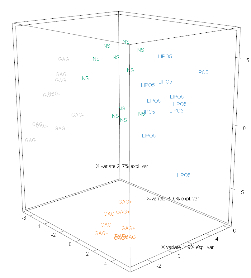
FIGURE 3: Sample plot for sPLS-DA performed on the vac18 data. Samples are projected into the space spanned by the first three components yielded by this method.
Variable Plots
A heatmap representation of each sample's feature values is very useful in this context. This has been visualised in Figure 4. The left-most column of colours depict the subject associated with each sample. It is of note that samples from the one subject were rarely clustered together (using hierarchical clustering) as seen in the dendrogram on the left. This once again shows how the multilevel approach avoids focusing on the inter-sample variation which usually does not yield any useful information.
# set the colours used for the subject assocaited
# with each sample (left-most column)
col.ID <- c("lightgreen", "red", "lightblue", "darkorange",
              "purple", "maroon", "blue", "chocolate", "turquoise",
              "tomato1", "pink2", "aquamarine")[vac18$sample]

cim(final.splsda.multilevel.vac18,
    row.sideColors = cbind(color.mixo(c(vac18$stimulation)), col.ID),
    row.names = paste(vac18$stimulation, vac18$sample, sep = "_"),
    col.names = FALSE, legend=list(legend = c(levels(vac18$stimulation)),
    col = c(color.mixo(1:4)),
    title = "Stimulation", cex = 0.8))
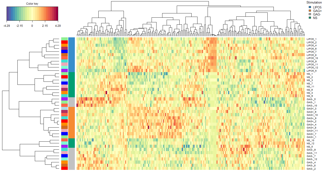
FIGURE 4: Clustered Image Map from the sPLS-DA performed on the vac18 data. The plot displays the genetic expression levels of each measured feature for each sample. Hierarchical clustering was done with a complete Euclidean distance method. The left-most column of colours denotes which subject a given sample belongs to. The colour column to the right of this shows the treatment associated with each sample.
More information on Plots
For a more in depth explanation of how to use and interpret the plots seen, refer to the following pages: